A compound pendulum under the action of uniform gravity is simulated using Multibody Dynamics and the Finite Element Method (MbDFEM). The objective is to determine the stresses induced in the material, resulting from the motion dynamics (force and torque) generated at the hinge joint.
The video on the left shows the final results of the pendulum MbDFEM simulation.
The video on the left shows the final results of the pin MbDFEM simulation, which are detailed in our next example.
The assembly is composed of two FreeCAD App::Parts:
The image on the left shows the pendulum (left) and pin (right) drawings and dimensions. The image below shows the isometric view of the Pin and Pendulum CAD geometries, and the global inertial coordinate system.
A material is assigned to both parts. Average steel was used for this example. From the CAD geometry and the assigend material, the physical properties of both parts are computed.
The tables on the left show the properties of the pin and the pendulum.
The table below contains the average properties of steel.
The pin is grounded (all 6 degrees of freedom are fixed to the global inertial coordinate system).
Earth gravity (9.807 m/s^2) is pointing in global negative Y direction.
The pin and pendulum each have one joint marker attached.
A hinge joint is defined between the two markers. This joint ensures that:
The image on the left shows the pendulum initial assembly and the direction of gravity. The images below show the markers and joint connector (left) and the solved assembly (right).
The pre-processor generates an input file for the MbD solver, This file uses *.mbd format. The MbD solver is launched. The results of the MbD simulation are stored as properties of the FreeCAD parts and joints, and saved in the *.FCStd. file. For each part, the following data are stored:
For each joint, the following data are stored:
The video on the left shows the pendulum motion.
The video on the left depicts an animated free-body diagram of the pendulum. It includes:
Force vectors are depicted by red lines. Torque by blue lines.
Here, the FEM simulation is applied to the Pendulum.
FreeCAD meshes the pendulum using Gmsh. For this example, a coarse mesh composed of tetrahedron elements is used.
Two FEM "bearing loads" are applied to the mesh at the hole of the hinge joint.
The first is from the hinge joint reaction force.
The second is from the hinge joint reaction torque. In this case, joint torque is zero.
These loads are automatically distributed among adequate nodes on the joint hole surface.
The
d'Alembert principle
ensures the pendulum FEM model is in static equilibrium throughout all the time steps. For this, the total acceleration vector at the
center of mass of each tetrahedron mesh element is computed,
and the negative of this acceleration is applied to each volume element in the FEM mesh.
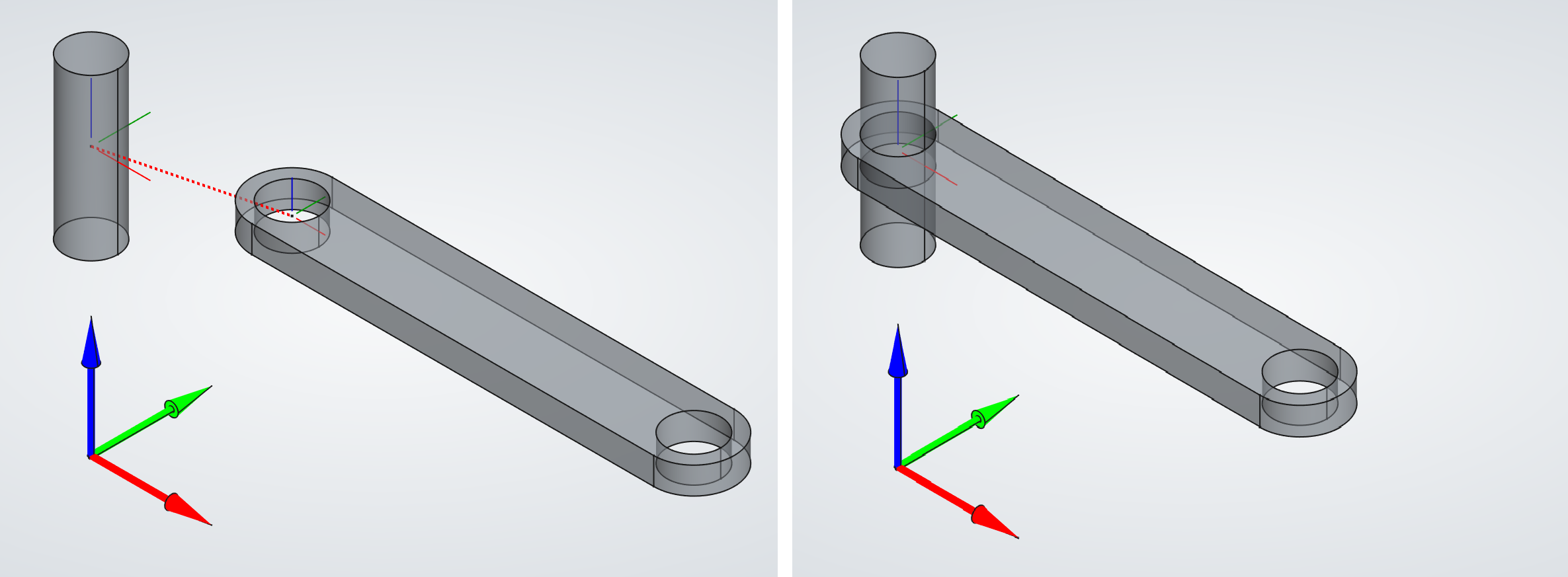
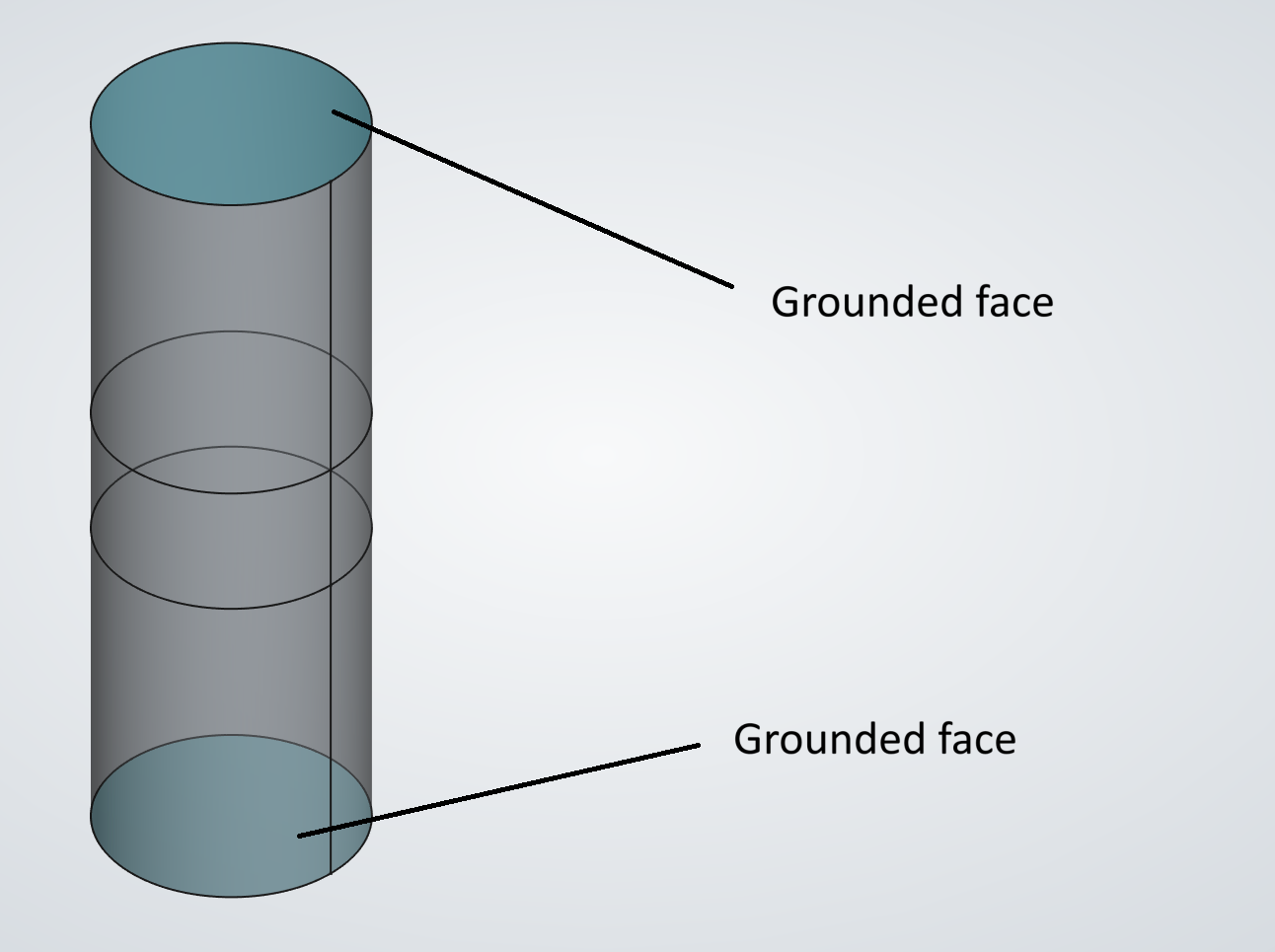
To prevent rigid-body motion, the pre-processor authomatically chooses three suitable nodes and applies fixed boundary conditions
using the "3-2-1" approach.
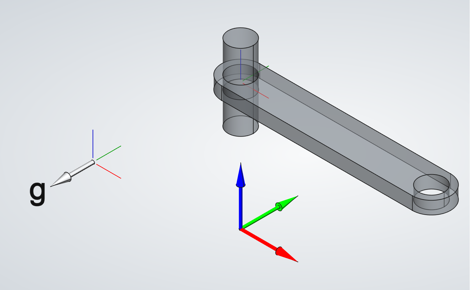
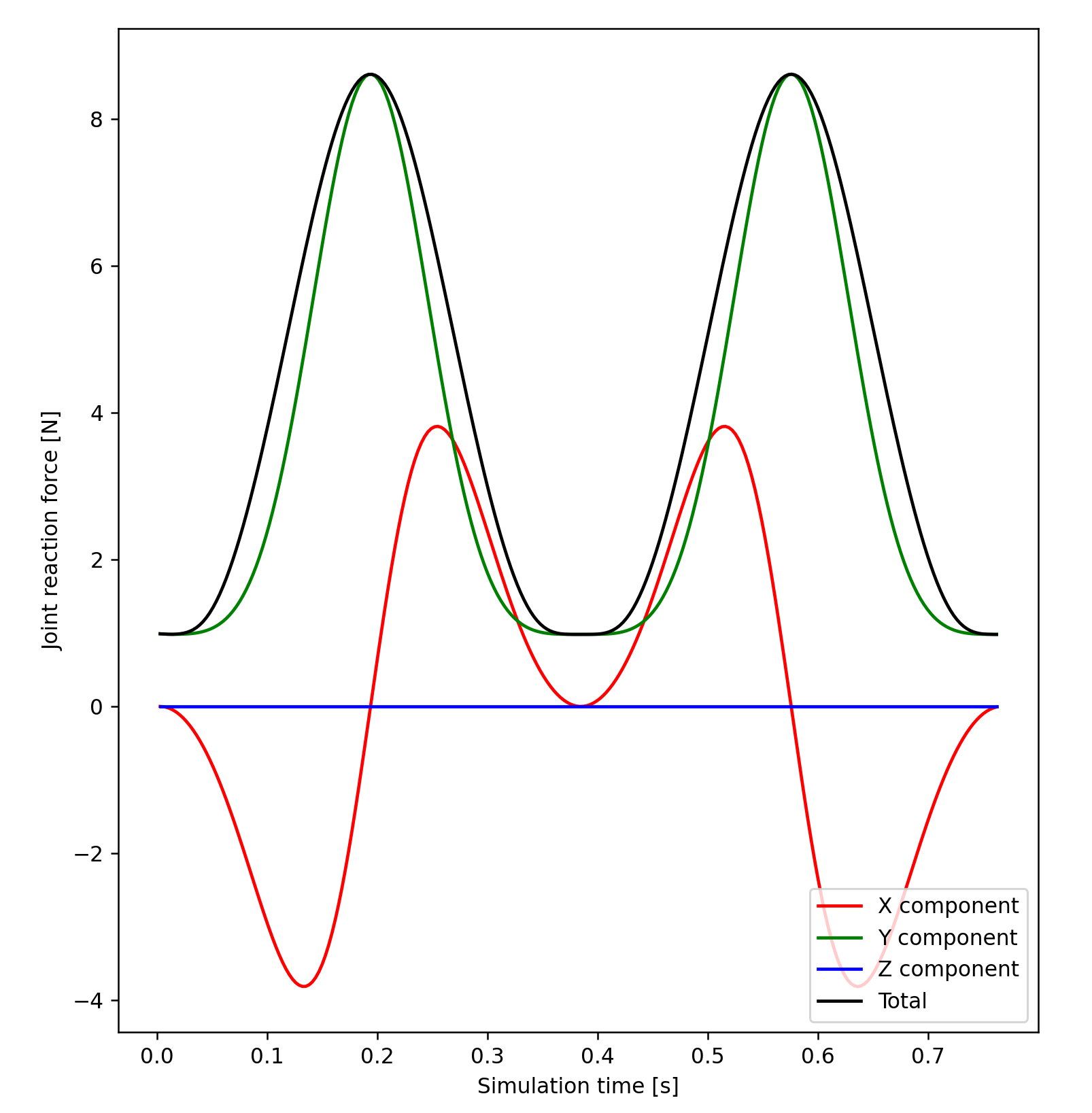
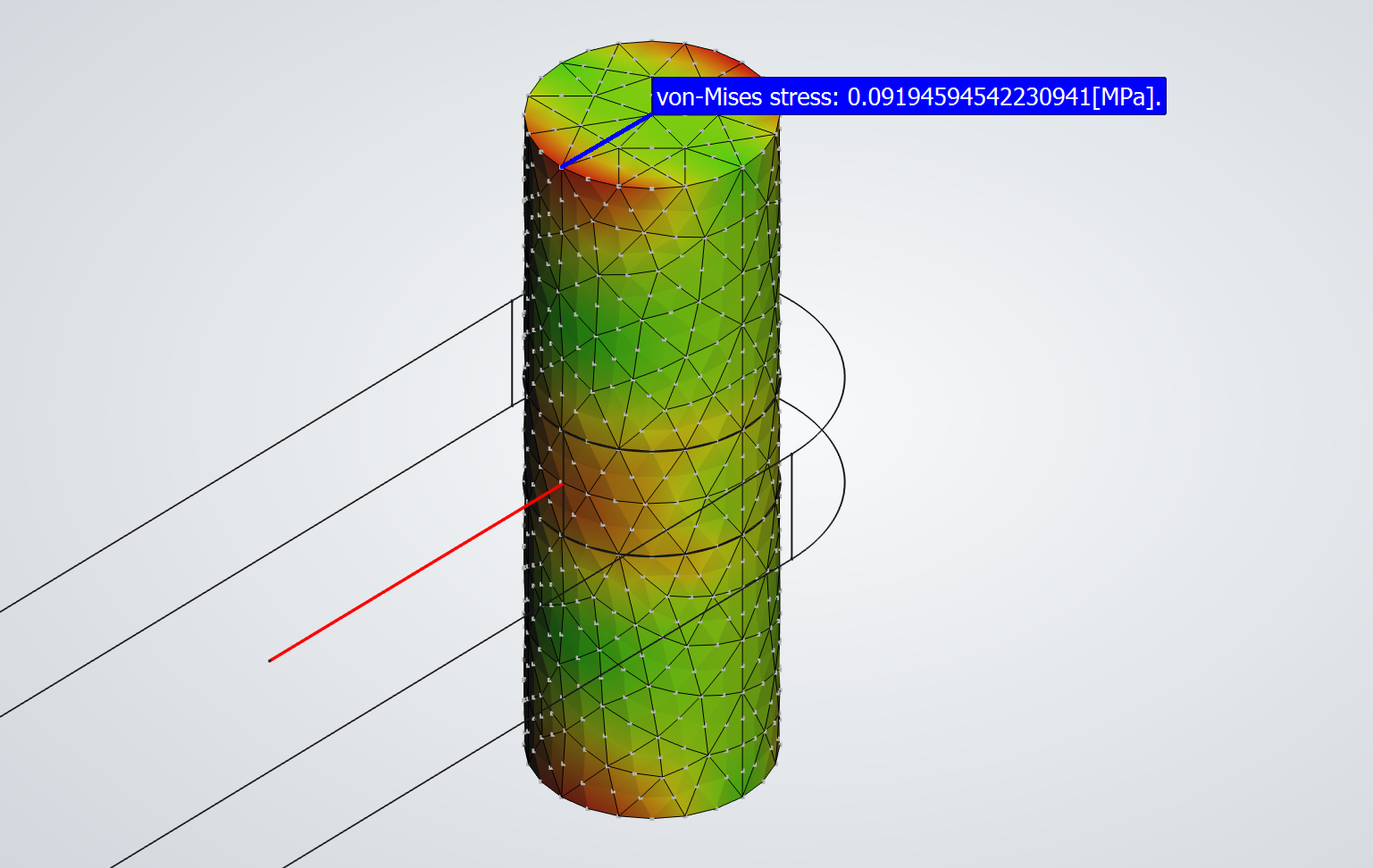
The video on the left shows:
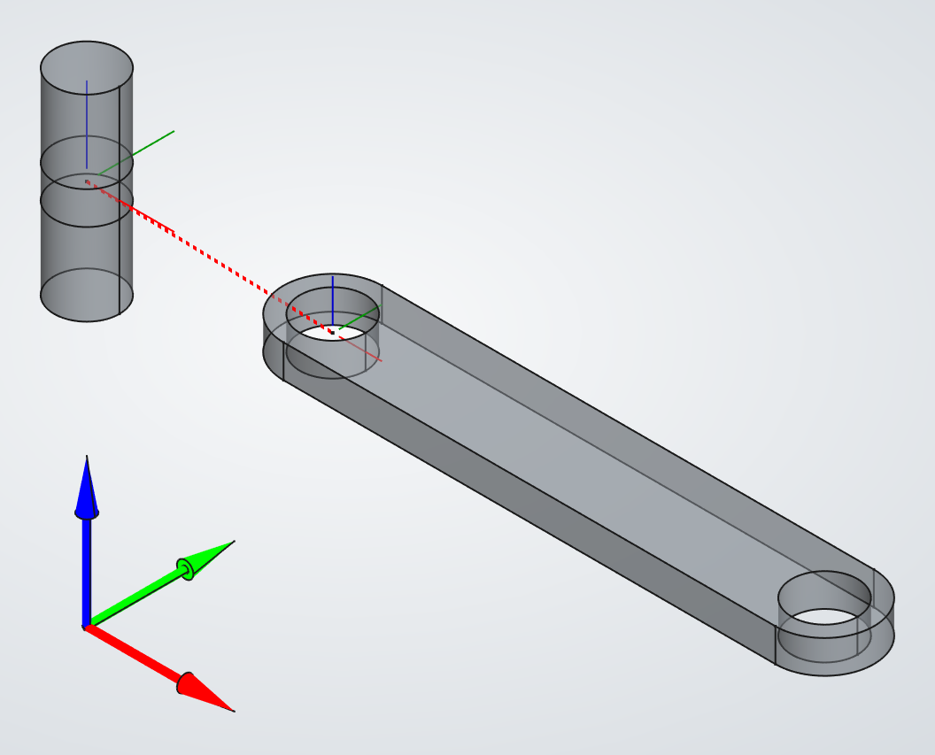
Load vectors are depicted by red lines. Acceleration vectors in orange.
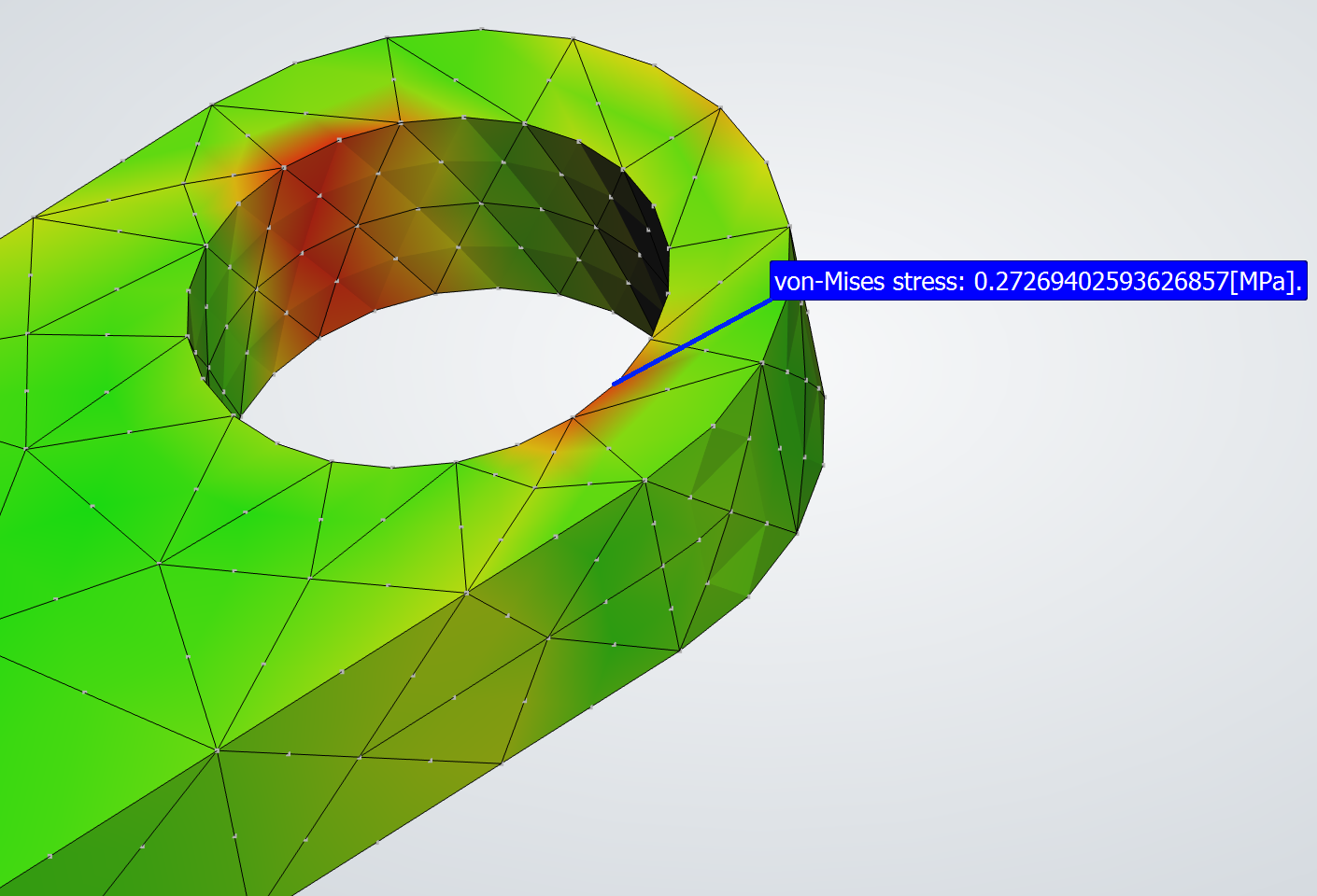
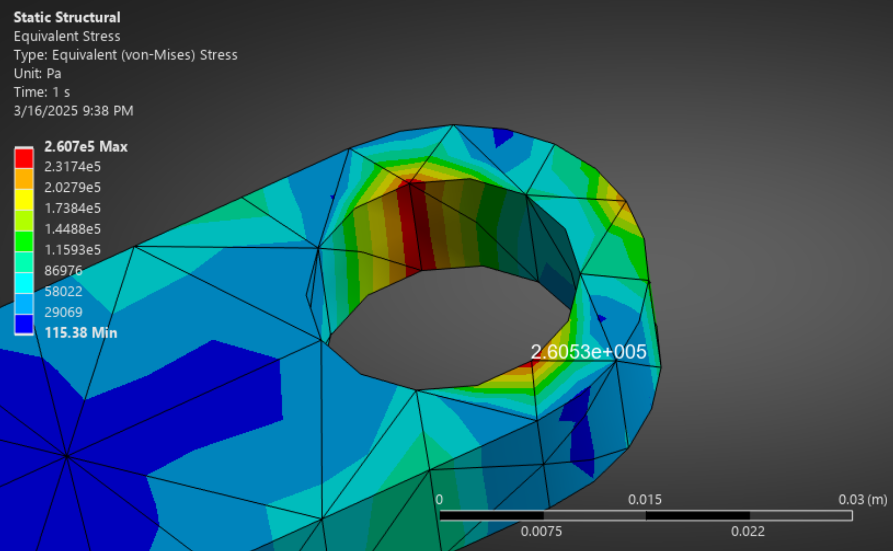
The pre-processor generates a set of input files for the FEM solver, one for each time step of the MbD simulation.
These files are in *.inp format.
The FEM solver is launched, solving the set of input files.
The results of each FEM simulation are stored as properties of the FreeCAD mesh object, and are saved within the *.FCStd file. These results include:
The MotionView post-processor allows the user to:
The video on the left shows the results of the MbDFEM simulation. The contour plots represent von-Mises stresses. The joint force vector is show for clarity.
One way to validate the simulation is to compare the reaction forces that take place at the nodes used for 321-constraint; with the joint loads applied to the FEM nodes. If the computation of the d'Alembert accelerations is correct, then the pendulum must remain in static equilibrium through all the time steps. Then, the 321-constraint nodes must see no reaction force. In reality, due to error introduced during numeric approximations, the reaction forces at the 321-constraint nodes must be a small fraction of the joint loads.
The plot below shows the joint force, while the plots on the left show 321 forces. One can see that the 321-constraint forces are three orders of magnitude less than the applied joint loads.
A second way to verify the simulation is to inspect the stress around the nodes used for 321-constraint. If the 321-constraint forces were a significant fraction of the applied loads, then the FEM solver would return a significant stress at the 321-constraint nodes. However, the stress at 321-constraint nodes is negligible compared to the stress produced by the joint load, as can be seen in the contour plots.
A third way to verify the simulation is to perform an equivalent simulation using another software. The pendulum was simulated using Ansys Mechanical. The images on the left and below (Ansys) show that both programs produce equivalent stress distribution, and that the maximum stresses occur at the same points and present a negligible difference.
Here, the FEM is applied to te pin. The CAD model and the dimensions of the parts, the initial conditions, the definition of gravity, and the MbD and FEM solver settings remain unchanged.
The video on the left shows the final results of the pin MbDFEM simulation.
In this simulation:
In order to have a face where the joint force is applied, the cylindrical face of the pin CAD geometry was split as shown in the image on the left.
All the FEM nodes belonging to the two circular faces of the pin were grounded, as shown below:
The video on the left depicts the joint force acting on the pin.
The video below shows the joint force load distribution among the FEM nodes.
The video on the left shows the von-Mises stress on the pin. The joint force vector is shown for clarity. The image below shows an isometric view of the frame and node of maximum stress.